Health care utilization is over-estimated in high-income regions that include low-income households. And individual income is over-estimated for low-income individuals living in high-income regions. Both lead to spurious conclusions, the former in studies of geographic variation and the latter in risk adjustment. This is a bit arcane, but it’s critically important, so read on……………

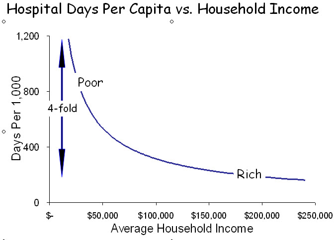
The most powerful characteristic associated with wellness, mortality and health care utilization is income. Low-income patients are sicker, die earlier and consume 2-4 times as much health care as affluent patients. And, because income inequality is greater in the US than in any other developed country, the extremes are greatest in the US.

Aside from its devastating social consequences, these circumstances present a challenge for risk adjustment. While some factors associated with poverty are captured by measuring severity of illness and co-morbidities, others are not. Examples include the effects of a nurturing childhood, adequate education and language skills; the impact of a caring environment with adequate physical resources and available care-givers; access to grocery stores, medications and transportation; safe neighborhoods; racial equality; and myriad other elements of life that impact on wellness, disease and healing. Many are a direct consequence of low income. Others are manifestations of poor neighborhoods – “poverty ghettos.” All correlate generally with income, even though income is not a measure of wealth, particularly in retirement, nor does current income necessarily reflect childhood income, which impacts on lifelong health. Despite these limitations, income is the index of importance.

How, then, to correct for income? Survey studies, such as the Medical Expenditure Panel Survey, include specific information about personal income, but most do not. Some studies of Medicare patients include Social Security income, a poor surrogate for personal income. Most studies lack specific information and rely, instead, on ZIP code income; i.e., the average income of individuals or households within the ZIP code of residence.

There are approximately 43,000 ZIP codes in the US. If the population were dispersed equally, each would have 7,500 people, but ZIP code populations range from fewer than 100 to more than 50,000. Moreover, because ZIP codes are formulated around mail routes rather than sociodemographic characteristics, many include individuals with a range of incomes. The errors that result from the use of ZIP code income are of two types: 1) high-income ZIP codes that include low-income residents are seen as utilizing more health care resources than their average incomes would predict (the geographic error); and 2) low-income residents of ZIP codes that include high income residents are assumed to use fewer resources than their actual incomes would predict (the risk-adjustment error). These two errors confound individual risk adjustment (as in hospital comparisons) and geographic risk adjustment (as in studies of regional variation).

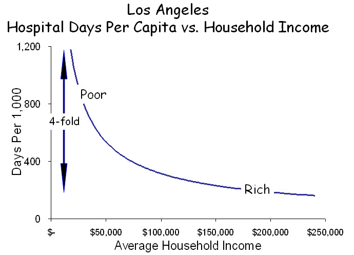
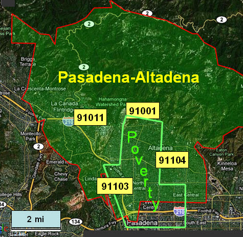
Los Angeles is a case in point. While it possesses a dense poverty core and several affluent zones, it is a patch-quilt of wealth and poverty, often juxtaposed. The Pasadena-Altadena area is one patch in this quilt. A small concentration of poverty overlaps four adjacent ZIP codes, each with more than 20,000 people. In all, this area has 46,000 households with a median income of $60,000, but median incomes among the four ZIP codes range from $36,000 to $110,000, and individual households within them have incomes ranging from $10,000 to more than $1.0M. The utilization of hospital care also ranges widely among these ZIP codes, from 205 days per 1,000 in the wealthiest to 1,045 per 1,000 in the poorest.

How does the mix of affluence and poverty within ZIP codes affect the determinations of health care utilization?  The figure below displays the income distribution in these four ZIP codes. From studies such as the graph above, we know that low-income households (shaded) contribute disproportionately to utilization and that utilization increases steeply at the lowest incomes. In contrast, high-income households contribute much less to utilization but contribute strongly to determining income.

The figure below illustrates the distribution of income in the four ZIP codes and indicates their average levels of hospital utilization. Utilization is influenced most strongly by the low-income households. Conversely, median incomes are influenced most strongly by high-income households. ZIP codes containing such mixtures of affluence and poverty form the “elbow” in the graph at the top. In ZIP 91011, which is predominantly high-income, the smaller proportion of low-income households contributes little to median income but disproportionately to average utilization. Only in ZIP 91003, with its predominance of low-income households, can a valid comparison be made between income and utilization. The consistent error is that utilization appears to be greater relative to income when higher-income ZIP codes include appreciable numbers of poor households. Aggregating and averaging such ZIP codes into hospital referral regions, as occurs in the Dartmouth Atlas, magnifies the error. In this way, affluent regions that include pockets of poverty, as most urban areas do, appear to use excessive resources, and because outcomes among the poor are poor, these resources are seen as “wasted.”

Risk adjustment is affected in the opposite direction. Because of where they live, low-income patients are assumed to have higher incomes than they actually have, sometimes very high, and adjustments that are  based on their assumed incomes fail to fully account for the added risk among low-income patients. This phenomenon is clear in the figure above. Depending on their ZIP code of residence, patients with low incomes will be viewed as wealthy, middle income or poor, and their “adjusted” utilization will be determined accordingly. The result is that, by under-correcting for risk associated with low income, hospitals that care for the poor are seen as “wasteful.”

These vagaries of household incomes within ZIPs cast a shadow over geographic comparisons of health care utilization and outcomes, and they raise serious concerns about risk adjustment applied to individual patients. It is important, therefore, to examine ZIP codes  to determine whether what they report about geographic variation is valid and, if not, to modify the analyses accordingly. No such remedy other than actual knowledge of patients’ incomes exists for risk adjusting individual patient experiences. ZIP code income is simply not a valid estimate. Hospitals that employ such an metric, as most must, will over-estimate  income for poor patients and under-adjust for risk.